Comparing SQL and Pandas for Data Analysis
Leveraging SQL and Pandas to extract insights from diabetes patient records

We will work with a dataset containing information on patients who have been diagnosed with diabetes or who do not present the condition. Our goal is to extract a sample of this data focusing on patients over 50 years of age. For each individual in this subset, we need to add a new column specifying whether the patient is classified as normal, with a Body Mass Index (BMI) below 30, or obese, with a BMI of 30 or higher.
Once the data is manipulated, it will be exported to a new CSV file and forwarded to the data scientist responsible for further analysis.
To address this task, we will use databases, Python, and SQL. Initially, the data will be imported using Python. Then, we will create a replica of this data in a database, where we will perform the necessary transformations using SQL queries.
After completing the required alterations and additions, the data will be transferred back to a Pandas dataframe, and finally, we will save the resulting dataset in CSV format.
We will use the Pima Indians Diabetes Database, a publicly available dataset downloadable here:
Pima Indians Diabetes Database
Overview
I am presenting to you a tutorial where we will extract and analyze data from databases — something incredibly useful that you will frequently use in your daily work as a data analyst. I will teach you how to manipulate data from relational databases.
If you have a CSV file, a TXT file, or any other file containing data, you can load this file directly into a relational database. Afterward, you can access this database using Python and apply SQL queries.
In other words, you don’t need to program in Python to analyze the data. You simply load the data into the database, access it through the Python environment, and apply SQL.
At the same time, you can also use Python if you want to conduct a more specific analysis, such as statistical analysis, building a machine learning model, or even creating visualizations. Python becomes a powerful platform for data analysis, allowing you to either use programming or, for instance, SQL.
This is the objective of this project. I will also take the opportunity to compare SQL syntax with the SQL procedures in Pandas when working with Python. I will present the options, and then you will choose what you consider ideal for your daily data analysis tasks.
Shall we begin?
Python Packages
The first step is to install the Watermark package. As the name suggests, this package allows you to create a watermark, which we will later use to record exactly which Notebook we are using, along with the versions of the installed packages and the Python version.
# 1. Install the watermark package
!pip install -q -U watermark
Note the exclamation mark at the beginning. This indicates that it’s an operating system command, not a Python command. The pip is the package installer for the language, and install specifies what I want to install.
The -q flag means quiet (silent installation), and -U stands for update—if the package is already installed, it will be updated. After that, comes the name of the package.
You can execute this either in the operating system, terminal, or prompt. If you want to run it here in Jupyter, just add the exclamation mark at the beginning and then click the Run button at the top. At that point, the package will be installed.
If the package is already installed, it will display a message saying so. Since I included the -q flag, no message will appear. If you want to see messages, simply remove the -q.
Additionally, for this project, I will also use the ipython-sql package, which is an excellent tool.
# 2. Install the iPython-sql package
!pip install -q ipython-sql
With this package, I will be able to use standard SQL directly to access data structures in Python. In other words, the same SQL you use directly in a database, outside of Python, can now be used here, within a Python data structure.
This is a huge advantage because SQL is almost a standard in the market when it comes to data analysis. Often, it is much easier to conduct analysis using SQL rather than building a Python script. Therefore, knowing how to do this within Jupyter is a great advantage, and this package will make our work easier — it’s the ipython-sql package.
After that, we will proceed with the imports.
# 3. Imports
import os
import pandas as pd
import sqlite3
I will use the OS package (Operating System) to handle system-level operations because I will need to manipulate filesand databases. I will also use Pandas, which is probably one of the most important Python tools for data analysis. Many people like to refer to Pandas as the Excel of the Python world, and it’s likely the most widely used software on Earth for this purpose.
With Pandas, you can replicate almost everything you do in Excel — though, in this case, you will need to write Python code. This gives you a lot of flexibility.
Regarding the database, I will use SQLite. So, we load the packages, and then, in sequence, we will also load the watermark extension.
# 4. Reload the watermark extension and display author information
%reload_ext watermark
%watermark -a "panData"
I will save showing the package versions for the end of the tutorial.
Creating the Relational Database
Now, let’s create our relational database. Follow along. First, I will create a dictionary.
# 5. Create a dataframe with the source data
data = pd.DataFrame({'level': ['Junior', 'Mid-level', 'Senior'],
                      'salary': [7500, 14650, 18320],
                      'position': ['Data Analyst', 'Data Scientist', 'Data Engineer']})
You see here? I know this is a dictionary because it opens and closes with curly braces. So, I have the key, followed by a colon, and the value is a list. Then, comma, key, colon, and the value is another list, and so on.
After creating this dictionary, I convert it into a table using Pandas, by calling the dataFrame function, which is a function from pd, the nickname we gave to Pandas.
# 6. List the data
data.head()
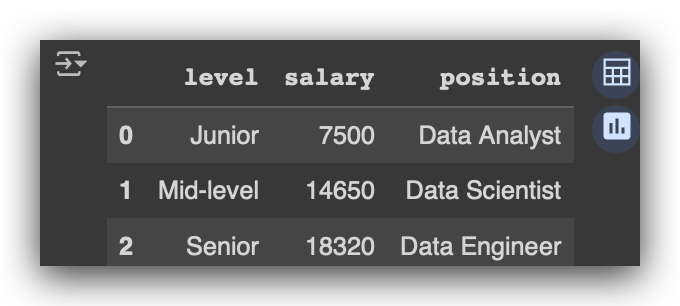
You then execute it, and next, visualize it using the head method. Now, you have a small table created in Python. This is a Pandas data structure, a table, or a dataFrame. But what am I going to do next? I will move this structure into a database so that I can work with it using SQL.
For that, I need to create the database. First, I’ll define the file name I want.
# 7. Define the path for the database file
file_path = 'database.db'
You can choose any name, as long as it has the .db extension. Here, I am defining the file name. Since I didn’t specify a folder, it will create this file in the same directory where the Notebook is located.
However, I added a conditional statement here for you.
# 8. Check if the file exists and delete it if it does, to create a new file later
if os.path.exists(file_path):
    try:
        os.remove(file_path)
        print(f"File {file_path} deleted successfully!")
    except Exception as e:
        print(f"Error deleting the file {file_path}. Details: {e}")
else:
    print(f"File {file_path} not found.")
If the file already exists, it will be deleted. If it doesn’t exist, it will create the file. What’s the advantage of this?
Every time you run the code, you will have a brand new database. From this fresh database, we will load it and begin our analysis.
Connecting to the Database with Python
Now, we will create a new database, connect to it, and then load the exact DataFrame we previously created into the database. From there, we can begin our analysis process.
# 9. Create the connection to a SQLite database
cnn = sqlite3.connect('database.db')
I will call SQLite3, which is the name of the package, and then use the connect method. This will attempt to connect to the database file. But you might wonder—how can you connect if you deleted the file?
Here comes the magic. This command will check if the file exists. If it does, it will connect. If it doesn’t, it will create the file and then connect. Yes, it’s really that simple, in just one line of code.
In fact, this is so easy that you need to be cautious — it can be dangerous. You might not want to lose your database, or you might not want to overwrite it by accident. You need to be careful, as it’s that easy.
In our case, I took the precaution of deleting the file first, so that I can now connect. If it doesn’t exist, it will first create it.

Notice that I placed this in the variable cnn, which is an SQL object. Go check the disk, and you'll see that the file was created. Observe the file size—Zero bytes. This means it’s an empty file, a completely blank database.
You can create a database and store whatever data you need inside. After that, you can perform your analysis using SQL. Alternatively, you can even use this as a way to backup your data. For instance, imagine you’re working on a project. You saved the results in a CSV file, sent it to the decision-maker, but you want to keep a copy.
If you don’t want to save it in CSV, you can save it in a database, which you can later access via SQL. Or, if you have a file that needs to be analyzed quickly, and there’s no time to create a Python script — no problem. You can load the file into the database and immediately apply SQL to analyze it.
This provides a huge advantage when it comes to data analysis.
# 10. Copy the dataframe into the database as a table
data.to_sql('employees', cnn)
Next, I will take the data object, and where did this object come from? From earlier—it’s the DataFrame. I will take the DataFrame and call the to_sql method. This method will take the contents of the DataFrame and transfer them to cnn. And what is cnn? It’s our connection, the connection to the database file.
When the data is transferred, it will create a small table called Funcionários (Employees). In other words, it will take the contents of your DataFrame, store them in the database, and in doing so, it must structure the data. It will create a table named employees.
# 10. Copy the dataframe into the database as a table
data.to_sql('employees', cnn)

The procedure was completed successfully. What is this number 3? It’s the number of rows in the table. After that, I will load the SQL extension using the package we installed earlier, ipython-sql.
# 11. Load the SQL extension
%load_ext sql
Then, you add %load_ext to load the SQL extension. This is also magical, alright? It’s even referred to as a magic command because it’s so seamless.
# 12. Define the database
%sql sqlite:///database.db
Then, you execute it, and now I’ll tell you the next step. I want to use that file as my database. So, I enter %sql, specify sqlite, which is the framework we are using to access the database, and then the file. In this case, I’m not specifying a folder because the file is in the same directory as the Notebook.
That’s it. Now you can start applying SQL using %%sql.
# 13. Execute SQL query to select all data from the employees table
%%sql

SELECT * FROM employees
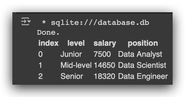
Be careful — you need to use two percent signs. Here, I am telling the Notebook the following: “Now, I don’t want to run Python code.” You see, the Notebook was created to execute Python. But for a moment, let’s pause Python and run SQL instead. That’s exactly what %%sql does.
Then, you enter your SQL instruction: SELECT * FROM, followed by the name of the table, which is employees, and the magic happens. Now you can work with SQL.
Since SQL is widely used in the industry, once you learn it, you can apply it in various contexts, projects, and in different ways. This is a quick method to analyze data without needing to write a Python script for it.
“Oh, but I don’t want to use SQL, I want to use Python scripts instead.” Can you? Yes, of course, that’s not a problem. However, the advantage of SQL is that it’s often a bit easier. SQL is not a programming language, it’s a data manipulation language. So you use SELECT to fetch everything from the source, which in this case is the employeestable.
Executing SQL Instructions for Data Analysis
Let’s execute a few more SQL commands as examples, and soon we will perform a complete data analysis. Let’s jump into the Notebook.
So, what have we done so far? We initially created a dictionary, converted it into a Pandas DataFrame, and then checked if the database file existed. Since the file didn’t exist, we deleted it to start fresh. Next, we connected to the database.
Since the file no longer existed, SQLite created a new file for us. After that, we loaded the table (which was the DataFrame) into the database under the name Funcionários (Employees). We then loaded the SQL extension, specified the location of the database (in the same directory as the Notebook), and executed our first query.
Here’s what you saw before:
# 13. Execute SQL query to select all data from the employees table
%%sql

SELECT * FROM employees
This SELECT * FROM employees, you execute here in SQLite. It's the same command you would run in Oracle, Microsoft SQL Server, IBM DB2, Teradata, MySQL, PostgreSQL, or any other database.
This is one of the great advantages of SQL — you learn one syntax, and you can use it across different platforms because SQL follows an international standard, which is SQL ANSI. This standard is supported by almost all database vendors.
So, what you’re doing here with me in Python, inside the Notebook, is the same as you would do in any other DBMS. Having this knowledge, which is interchangeable across platforms, is incredibly valuable.
Alright, now let’s run two more SQL commands. As an example, I want to count how many employees I have in the table.
# 14. Execute SQL query to count the number of records in the employees table
%%sql

SELECT count(*) FROM employees
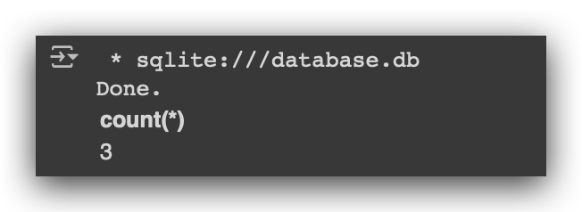
I will use the COUNT function, opening and closing parentheses and placing an asterisk inside. Done, I have three records.
If I want something a bit more complex, for example, what’s the average salary of the employees?
# 15. Execute SQL query to calculate the average salary rounded to 2 decimal places from the employees table
%%sql

SELECT round(avg(salary), 2) as 'average_salary' FROM employees
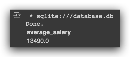
Next, I do this: SELECT, and I’ll use the AVG function, which is the average calculation in SQL. I then specify where I want to calculate the average. When calculating, it will return several decimal places. You can round it using the ROUND function to two decimal places. Then, you assign an alias using AS. This AS allows you to give a nickname to the result. You will do all of this based on the employees table.
Execute it, and there it is — the average salary. In other words, the only limit now is your knowledge of SQL. The more you know, the more you can extract from the database for analysis.
You don’t necessarily need to use Python for this analysis. If you know SQL, you can leverage it with any tool. On the other hand, if you don’t know SQL, or don’t want to use it, we can achieve the same result using Python.
In a moment, I’ll show the difference between Pandas syntax in Python and SQL syntax. But now, let’s load the CSV file and move it into the database.
Loading a Database from CSV Files
This is one of the greatest advantages of using SQLite with Python programming. You can take the contents of a CSV, TXT, or any other file and load them directly into the database, allowing you to perform analysis right here in the Notebook.
Here’s how we will do this.
# 16. Load the dataset
df = pd.read_csv('dataset.csv')
I will use the read_csv function from Pandas to read the dataset.csv file. This data contains information about patients who became pregnant and whether they developed diabetes or not. We will load this file into a DF, which is a Pandas DataFrame. I am loading the files using Pandas.
# 17. Check the type of the dataset
type(df)

Let’s take a look at the type of this object. You’ll see that it’s a DataFrame, which is essentially a table in Pandas. It’s the same concept you have in Excel, for example. Now, let’s check the shape.
# 18. Get the shape of the dataset
df.shape
We have 768 rows and 9 columns. Let’s take a look at a sample of the data using the head method.
df.head()

So, we have the number of times the woman was pregnant, glucose levels, blood pressure, insulin levels, and the BMI (Body Mass Index). We also have the age and the outcome, which indicates whether the patient (in this case, a female) developed diabetes or not.
Now, I will take this table and move it into the database.
# 19. Copy the dataframe into the database as a table
df.to_sql('diabetes', cnn)
So, I take the DF and call the to_sql function. I will load this into cnn, which is our connection to the database file (which is still open). This will create the diabetes table. In other words, you can create as many tables as you want.
Notice that we already have a table, right? The employees table, which we loaded into the database earlier from our small initial dataset. Now, I will create another table in the database, but this time from the CSV file.
You can add multiple tables to your SQLite database, each associated with a different project or dataset, and so on. Let’s execute, and done! You’ll see the number 768 appear, which corresponds to the number of rows. The table has been successfully created in the database.
Now, we can start using SQL. I will count the records to make sure everything is correct in the database.
# 20. Execute SQL query to count the number of records in the diabetes table
%%sql

SELECT count(*) FROM diabetes
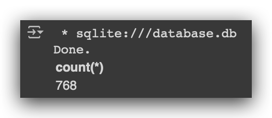
Done! Look at that — 768 rows, and the table was created successfully. You can use this to backup your data, or, for example, you can store your data in the database and later analyze it using SQL. You can even save the results of your work directly in the database and send it via email.
Yes, absolutely. You can take the .db file, attach it to an email, and if you want, you can zip it. How cool is that? You can send the database through email — definitely, we are living in a new world where databases travel over the internet via email.
So, if you need to share this data with someone from your team or a client, you can directly send the database file itself. That’s pretty neat.
Now, I’ll show you the difference between SQL syntax and Pandas syntax.
SQL Syntax vs. Pandas Syntax
Now, I will show you the difference in syntax when you use Pandas to query data versus when you use SQL to query the database.
For example, imagine I want to create a query that returns the patients with a BMI (Body Mass Index) greater than 52 and an age between 25 and 30 years. I need to retrieve these patients for further analysis.
We can use the following Pandas syntax for this:
# 21. Pandas query
df.query("BMI > 52 and 25 <= Age <= 30")
What is the DF? It’s our DataFrame, which is essentially a table. I call the query method: DF.query. I open parentheses (because the method is a Python function) and, in quotes, I specify the rule or condition to filter the data.
Notice that I am stating which table I’m working with (df), then specifying the columns (BMI and age), and concatenating the rules. So, BMI greater than 52, and (and being the logical operator) age greater than or equal to 25 and less than or equal to 30.
Then, you execute it.

How would we do the same thing using SQL?
# 22. SQL query
%%sql

SELECT * FROM diabetes WHERE BMI > 52 AND Age BETWEEN 25 AND 30
Like this: SELECT * FROM diabetes, which is the table in the SQLite database. The WHERE clause applies the row filter—where BMI is greater than 52, and (AND, the logical operator) age is between 25 and 30 (BETWEEN is used to specify a range).
Now, compare that for me.

See if the result isn’t exactly the same. Same outcome? Excellent. The first query we executed directly on the Pandas DataFrame. The second one was done on the database table.
Now, I imagine you have two questions, right? The first one is quite logical: why would I use this SQL query if I can achieve the same result with less code in Pandas? Why should I use SQL here?
Well, for a very simple reason: this Pandas query only works with Pandas — it’s exclusive to Pandas and only functions there. On the other hand, the SQL query works in any DBMS (Database Management System). So, you might be querying data on another platform, and for some reason, you come into Python for further analysis. You can use the exact same query.
In other words, you could use this query in Oracle, MySQL, CERN, DB2, Teradata, PostgreSQL, MySQL, and so many other systems. This is a huge advantage, isn’t it? Because once you learn SQL, you can use it on many different platforms.
Of course, the Pandas syntax is a bit simpler, but it will only work with Pandas. Do you get the idea? It’s not about one being better or worse — it’s purely about analyzing the data.
Personally, I prefer SQL a lot, because I can write my query here, and later I can take the same query and use it on any other platform.
That’s the first point. The second point, which will also help you decide which one to use in your daily tasks, is about performance. Here, we have fewer than a thousand records, but what if we had a million records or even a billion?
Pandas has certain limitations in terms of memory usage. When you work with databases, you have additional resources, such as index creation, table partitioning, auxiliary table configuration, and constraints that enforce rules in the database. All of these can help improve performance and provide greater security.
So, in general, SQL gives you more tools to create better-performing queries.
Why would you still use Pandas? Because sometimes you might not have a database or the means to create one at the moment, and you need to deliver an analysis quickly. Why not use Pandas in this case? Your goal is to perform the analysis, not to choose tool A or B.
Is it a quick analysis? Maybe it doesn’t make sense to create a database, load the data, and run the query there. In that case, I would use Pandas.
On the other hand, if you are going to perform a series of analyses, like we will soon, it might make more sense to put the data in a database and use SQL. It always depends on your objective and what you want to achieve in the final result of your project.
I’m showing you the difference in syntax so that you understand you have two options. Perhaps the best approach is to learn both, right?
Another advantage of Pandas syntax is that you don’t need to load the CSV file into the database. You can just load it into the Python environment and start querying it.
But if you need more performance, more customization, or to work with multiple tables, I would probably opt for SQLsince it’s more appropriate, more intuitive, and the same query can be used on other DBMS platforms.
Is that clear to you? Now, let’s do a complete data analysis using SQL with our database.
Business Questions with Data Analysis
I will present a situation, a scenario, and then we will solve the business problem using SQL with a database. Let’s go.
We need to generate a data sample of patients over 50 years old, and for each of them, we need to indicate in a new column whether the patient is normal (with a BMI, or Body Mass Index, of less than 30) or obese (with a BMI of 30 or higher). We will then generate a new CSV file and send it to the decision-maker.
First, I need to filter my table to retrieve only patients over 50 years old. Then, I will add a new column and define a business rule: BMI less than 30, the status is normal; BMI greater than or equal to 30, the status is obese. After that, I will save the result in CSV and deliver it to the decision-maker.
Did you get the scenario? Alright, let’s solve it.
The first step is to give you an example of how to create a query with a condition to apply a row-level filter. It’s basically like this:
# 23. Execute SQL query to return Age, Glucose, and Outcome for patients with Glucose greater than 195
%%sql
SELECT Age, Glucose, Outcome FROM diabetes WHERE Glucose > 195⬤
You return the columns you want using SQL. If you use *, it will return all the columns. If you don’t want all of them, you must specify which columns you want. You indicate the table from which you want to pull the data and apply the filter with the WHERE clause. For example, glucose greater than 195.
This is just an example. Once the filter is applied, you get the data you need.
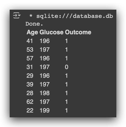
Notice that I applied the filter at both the column level and the row level, right? My diabetes table has several columns, but I filtered it to return only three. Similarly, my table has many rows, but I filtered it to return only those where glucose is greater than 195.
This demonstrates that it’s possible to filter at both the column and row levels. Now, stay with me.
# 24. List the columns of the dataframe
df.columns⬤

Here, I have all the columns from our DataFrame. Now, I’m going to do the following: I will create a new table in the database. Why? So that I can store the result of the business problem in this table.
This is where you start to see the advantages of using SQL. You can quickly create tables, filter data, and generate small samples. Later, you can use this for your own analysis or send it to the decision-maker.
# 25. Create the 'patients' table in the database
%%sql

CREATE TABLE patients (Pregnancies INT,
                       Glucose INT,
                       BloodPressure INT,
                       SkinThickness INT,
                       Insulin INT,
                       BMI DECIMAL(8, 2),
                       DiabetesPedigreeFunction DECIMAL(8, 2),
                       Age INT,
                       Outcome INT);
Now I will create a new table. If you enter %%sql and then use the CREATE TABLE statement to create the patientstable, you can define the columns and their data types. Inside this table, you will store the data.
Once the table is created, we will proceed with the SELECT query.
# 26. Execute SQL query to select all data from the patients table
%%sql

SELECT * FROM patients

To check if the table was created, we run the SELECT query. The table has been created, and it’s currently empty. All good so far?
So, I’ve created a new table, and now I’m going to populate it based on the business rules that we defined for this scenario.
Now, pay close attention to what I’m going to do next. I’ll increase the complexity a bit to ensure you get the most out of this and really expand your knowledge.
# 27. Insert data into the patients table for patients older than 50 years
%%sql

INSERT INTO patients(Pregnancies,
                     Glucose,
                     BloodPressure,
                     SkinThickness,
                     Insulin,
                     BMI,
                     DiabetesPedigreeFunction,
                     Age,
                     Outcome)
SELECT Pregnancies, Glucose, BloodPressure, SkinThickness, Insulin, BMI, DiabetesPedigreeFunction, Age, Outcome
FROM diabetes WHERE Age > 50;
Insert into. I am going to insert data into the patients table. This is what an SQL instruction looks like. What do I have in this patients table? These columns, right? So, I place them between parentheses.
And what am I going to insert into the table? Essentially, the result of the query shown below.
SELECT Pregnancies, Glucose, BloodPressure, SkinThickness, Insulin, BMI, DiabetesPedigreeFunction, Age, Outcome
FROM diabetes WHERE Age > 50;
In other words, I am concatenating two SQL commands. I will insert into the patients table the result of a query that fetches the data from each column of our diabetes table, but only where the age is greater than 50, which is the first rule of our scenario.
There are many ways to do this; I am showing one alternative. Now, let’s execute it.
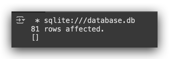
We’ve loaded the data. Done. 81 patients meet our criteria and are now in the patients table. To check, just run the SELECT query.
# 28. Execute SQL query to return all data from the patients table
%%sql

SELECT * FROM patients;
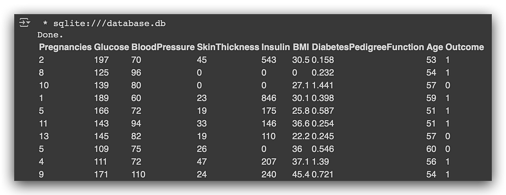
Look at that — 81 patients, following exactly the rule that age must be over 50. Notice the power of what we’ve done here. I can have a large dataset, a big database, and apply filters at both the column and row levels. This allows me to generate a smaller sample, move it into another table, and continue with my analysis.
Now, that’s exactly what we’ll do next. One of the rules we need to implement is to indicate in a new column whether the patient is normal or obese. So, I’ll need to create a new column, right?
# 29. Alter the patients table to add a new column
%%sql
ALTER TABLE patients
ADD Profile VARCHAR(10);
Now, I will use the ALTER TABLE command. So, I will alter the patients table. I will add a new column called Profile, which will be of type VARCHAR(10).
What does VARCHAR(10) mean? In this Profile column, you can store up to 10 characters. You can store 9 characters, 8, 7, or even none—but you cannot store 11 characters, because the limit is 10. The number of characters varies, hence varchar, but with a maximum of 10.
And just like that, you create a new column in your table. Let’s check to see if the column was created?
# 30. Execute SQL query to return all data from the patients table
%%sql

SELECT * FROM patients;

Let’s run a SELECT *. Look how nice—column created successfully. Why is there a None here? Because the column was created, but I don’t have any data in it yet. I only created the column. What does SQLite do? It fills the column with None.
And here’s a very important observation: what just happened is not a problem or an error. I created the column, but I haven’t populated it yet. Since there is no data, SQLite inserts None, which represents a missing value.
During your data analysis process, you might generate missing values like this. That’s why I always recommend that after each step in your data processing, you check the data. Each time you make a transformation, go back and check: Did I unintentionally create an issue? Did I possibly cause an error? Anything can happen — you’re not seeing all the data at once, right?
So, it’s always good to verify, which is why I’m showing you the SELECT * from the patients table to check what’s happening at each stage. In this case, I have everything under control. I created the column, and SQLite filled it with None, but that’s fine.
Now, I’m going to populate the column with data based on the business rule we have defined.
What do I need to do? I need to fill the Profile column based on the rule we have in our business case. So, let’s start by updating the column with the value ‘Normal’ if the BMI is less than 30. I will use the SQL UPDATE command again to update the table.
# 31. Update the Profile column with "Normal" where BMI is less than 30
%%sql

UPDATE patients
SET Profile = 'Normal'
WHERE BMI < 30;
The table is called patients. I will use the SET command. I will set the value of the Profile column to ‘Normal’, which is a string. But I will only do this where the BMI is less than 30.
Now, I’ll update the table.
# 32. Execute SQL query to return all data from the patients table
%%sql

SELECT * FROM patients;

Execute it, then run a SELECT, and look. Where the criteria are met (just look at the BMI column), you’ll see that it has been set to ‘Normal’. Where the criteria are not met, it remains None — excellent.
Now, I need to update the other part of this column, which follows the rest of the business rule.
# 33. Update the Profile column with "Obese" where BMI is greater than or equal to 30
%%sql

UPDATE patients
SET Profile = 'Obese'
WHERE BMI >= 30;
I will set the value to ‘Obese’ if the BMI is greater than or equal to 30. I’ll use the UPDATE command again, updating the table to set the value of the Profile column to ‘Obese’, but only where the BMI is greater than or equal to 30.
Execute it, and let’s check the content.
# 34. Execute SQL query to return all data from the patients table
%%sql

SELECT * FROM patients;
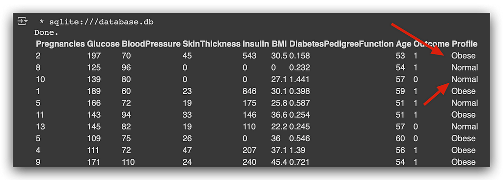
Notice that now the Profile column is fully populated. See how we used the power of SQL to quickly prepare a data sample? And what we just did — this UPDATE, INSERT INTO, SELECT, and any other commands — can be used in any other DBMS.
You learn SQL once and can use it on various platforms, which is why SQL is so valuable. I’ve always worked a lot with databases, and when you work with data science and data analysis, you’ll be working with databases all the time.
Even if you don’t use SQL directly, look at this — what is this? SQL. Do you think the folks at Pandas invented this from scratch? No. They looked at SQL syntax and thought: how can we bring this into Pandas? This is SQL in practice.
Remember, SQL was created in the 1970s. All these other tools came much later. So what the Pandas team did was simply adapt SQL syntax so you could use it directly with the Pandas package.
If you know SQL, you naturally gain a clear understanding of what’s happening. SQL becomes one of the main tools in your daily data analysis tasks.
Now, what do we need to do? Save this result as a CSV to send it to our decision-maker.
Delivering the Results of the Analysis to Decision-Makers
Alternative 1
We have now completed our work. We have the sample based on the business problem rules. So, now we have a table with patients over 50 years old, and we created the Profile column, where the value is ‘Normal’ if the patient’s BMI is below 30, and ‘Obese’ if the BMI is 30 or higher.
The data sample is ready, and I need to send it to the decision-maker. Well, we have a few alternatives. Here’s one for you.
# 35. Query
query_result = cnn.execute("SELECT * FROM patients")
I will take the cnn. What is cnn? It’s our connection — the connection to the database. The connection is still open.
I will then take the connection and call the execute method, which will execute something. What will I execute? An SQL instruction: SELECT * FROM patients, just like I did earlier. When I execute this instruction, it will return the entire table.
I will take this entire table and save it in the query_result. What will this object be? Let’s execute this line and find out.

Next, print the query_result. You’ll see that it’s an sqlite3.Cursor. What is a Cursor? It’s basically an object that allows you to iterate through all the data in the table. You can access all the rows and all the columns. This type of object is very common and has been around for decades.
You can access a database, return the entire table, place it in a cursor object, and then access it row by row, column by column.
Alright. Now that we have this object, I’ll create a List Comprehension.
# 36. List comprehension to return the table metadata (column names)
cols = [column[0] for column in query_result.description]
A basic repetition structure in Python. Read along with me, okay? For each column in the query description (the description contains information about each column), I will return the column at index 0.
What for? For this right here.
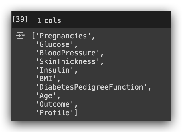
Execute the names of all the columns in the table. When you executed this command in cell #35, it returned the entire table. So, I can now iterate over the columns and over the rows.
What I did first was retrieve the name of each column. Now, here’s what I’m going to do next: I will retrieve each row and store them in a Pandas DataFrame.
# 37. Generate the dataframe
result = pd.DataFrame.from_records(data=query_result.fetchall(), columns=cols)
So, I will use pd.DataFrame.from_records. I will create a DataFrame from records. Where do these records come from? From my query_result, which is the cursor. I’ll call fetchall(), which retrieves all the rows. I want all the rowsfor all the columns.
Done. I’m fetching each row and each column and storing them in result.
# 38. Shape
result.shape
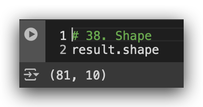
Check the shape: 81 rows and 10 columns. Let’s take a look at a sample.
# 39. Visualize
result.head()

See, I pulled the data from the database. Now, I’m back in the Python environment. I have a DataFrame. I can now save the DataFrame as a CSV file, making sure to set the index to False.
# 40. Save to CSV
result.to_csv('result.csv', index=False)
I don’t want the index, I just want the data. Done. I saved the file to disk. Let’s take a look, shall we? Open the CSVresult. You can now attach it to an email and send it to the decision-maker.
Now, you might say: I had to connect to the database, run the query, extract each column, extract each row, generate a DataFrame, and then save it as a CSV. It was quite a bit of work.
Is there an easier way to do this? This is the kind of question you should ask frequently. When faced with any situation in data analysis, ask yourself: Is there another way to do this? Is there a simpler way? Keep asking this question constantly.
Because now you will seek the answer: Yes, there is a much simpler way to do this, but I’ll need another tool. It’s a trade-off, right? You have to choose. You can do it here without any other tools, just with Jupyter Notebook, as I’ve just shown you.
Didn’t like this method? Think it’s too much work? If you want to make it simpler, you’ll need another tool.
Alternative 2
So, is there a simpler way to generate the CSV file to send to the decision-maker? Yes, there’s another alternative — actually, there are several alternatives, right? I’m going to show you another one now, which will require another tool, but it’s free, super easy to use, and very useful for your day-to-day tasks.
You could also send the database file, but the decision-maker probably doesn’t know how to manipulate that file. It’s not their job to know, right? For example, a marketing manager won’t know how to open a DB file. It’s not their job — it’s your job to make the decision-maker’s life as simple as possible.
We generated the CSV file, but we found it a bit tedious, right? Let’s do this: I’m going to use a tool that will access the database directly. I won’t use Notebook, I won’t use Python — I’ll access the DB file directly, and inside the tool, there’s a button that lets you generate the CSV file.
Want to check it out? Follow me. First, go to this website:
This is a free tool that you can download and install on your computer to access the SQLite database file. So, click here to download it. You’ll see that there are versions for Windows, macOS, and Linux. Choose the one that suits your system, download it, and install the tool.
Once it’s installed, open it. Take a look — this is the interface:
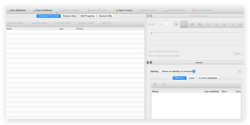
This is DB Browser for SQLite, which is essentially an interface to access your database file. Click at the top on Open Database, and it will open a dialog box. Then, navigate on your computer to find the DB file, select the file, and click Open.
Done! The file is open. Excellent. In other words, the database is open, and the tables we created — diabetes, employees, patients — will appear.
Double-click on patients. You’ll see all the columns, everything neatly laid out, ready for analysis. Now click on Browse Data, which is at the top.

Click there, and it will show you the contents of each table. Select the patients table, and look at the bottom — the footershows that there are 81 rows.
Now, click on this arrow here.
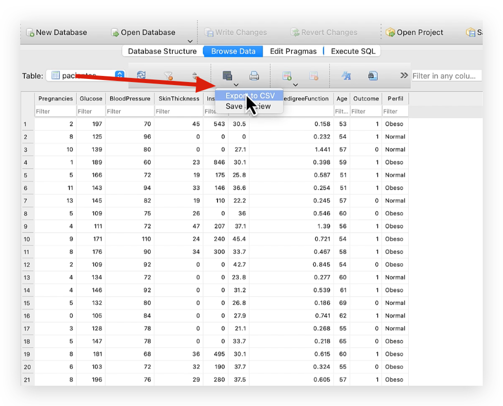
Click Export to CSV. It will show you the options for characters, column separators, row separators, etc. Then click Save, choose where you want to save the file — I’ll save it as resultado.csv with no issues, but you can create another copy or a different file if you prefer.
Click Save. It will ask if the file already exists and whether you want to overwrite it. Click Yes, Replace, and done. Export Completed. Excellent!
As you can see, DB Browser is very intuitive. Here, you can also build some SQL queries, modify columns, and rows, or even create a new database if you want. You can also visualize other tables. In short, it’s a very useful tool to have in your daily work if you ever need to access the database file directly.
This tutorial was just to get you started, to give you a small glimpse into the world of data analysis. We’ll meet again next time.
Thank you very much. 🐼❤️
All images, content, and text are created by Leonardo Anello
Comparing SQL and Pandas for Data Analysis was originally published in Towards Data Science on Medium, where people are continuing the conversation by highlighting and responding to this story.
from Datascience in Towards Data Science on Medium https://ift.tt/hBrxt7W
via IFTTT


