Using Objective Bayesian Inference to Interpret Election Polls
How to build a polls-only objective Bayesian model that goes from a state polling lead to probability of winning the state
With the presidential election approaching, a question I, and I expect many others have, is does a candidate’s polling in a state translates to their probability of winning the state.
In this blog post, I want to explore the question using objective Bayesian inference ([3]) and election results from 2016 and 2020. The goal will be to build a simple polls-only model that takes a candidate’s state polling lead and produces a posterior distribution for the probability of the candidate winning the state
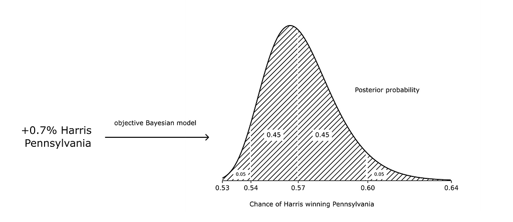
where the posterior distribution measures our belief in how predictive polls are.
For the model, I’ll use logistic regression with a single unknown weight variable, w:

Taking the 2020 and 2016 elections as observations and using a suitable prior, π, we can then produce a posterior distribution for the unknown weight

where

and use the posterior to form distributions for prediction probabilities

where X̃ denotes state polling lead, P̃ denotes the probability of the leading candidate winning the state, and φ denotes the inverse of the logistic function, the logit function:

Let’s turn to how we can construct a good prior using reference analysis.
How to derive a prior with reference analysis
Reference analysis ([3, part 3]) provides a framework to construct objective priors that represent lack of specific prior knowledge.
In the case of models with a single variable like ours, reference analysis produces the same result as Jeffreys prior, which can be expressed in terms of the Fisher information matrix, I:

For single variable logistic regression, this works out to

π(w) will be peaked at 0 and will approach an expression of the form

as |w| -> ∞, making it a proper prior.
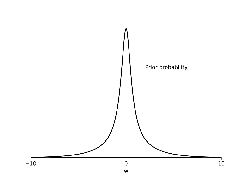
Let’s run a quick experiment to test how well the prior represents “knowing nothing”.
from bbai.glm import BayesianLogisticRegression1
import numpy as np

# Measure frequentist matching coverage
# for logistic regression with reference prior
def compute_coverage(x, w_true, alpha):
    n = len(x)
    res = 0

    # iterate over all possible target values
    for targets in range(1 << n):
        y = np.zeros(n)
        prob = 1.0
        for i in range(n):
            y[i] = (targets & (1 << i)) != 0
            mult = 2 * y[i] - 1.0
            prob *= expit(mult * x[i] * w_true)

        # fit a posterior distribution to the data
        # set x, y using the reference prior
        model = BayesianLogisticRegression1()
        model.fit(x, y)

        # does a two-tailed credible set of probability mass
        # alpha contain w_true?
        t = model.cdf(w_true)
        low = (1 - alpha) / 2
        high = 1 - low
        if low < t and t < high:
            res += prob
    return res
This bit of python code uses the python package bbai to compute the frequentist matching coverage for the reference prior. We can think of frequentist matching coverage as providing an answer to the question “How accurate are the posterior credible sets produced from a given prior?”. A good objective prior will consistently produce frequentist coverages close to the posterior’s credible set mass, alpha.
The table below shows coverages from the function using values of x drawn randomly from the uniform distribution [-1, 1] and various values of n and w.

Full source code for experiment: https://github.com/rnburn/bbai/blob/master/example/22-bayesian-logistic1-coverage.ipynb
We can see that results are consistently close to 0.95, indicating the reference prior performs well.
In fact, for single parameter models such as this, the reference prior gives asymptotically optimal frequentist matching coverage performance (see §0.2.3.2 of [4] and [5]).
Using the reference prior, let’s now take a look at how predictive polls have been in previous elections.
2020 Election
Here’s how FiveThirtyEight polling averages performed in 2020:
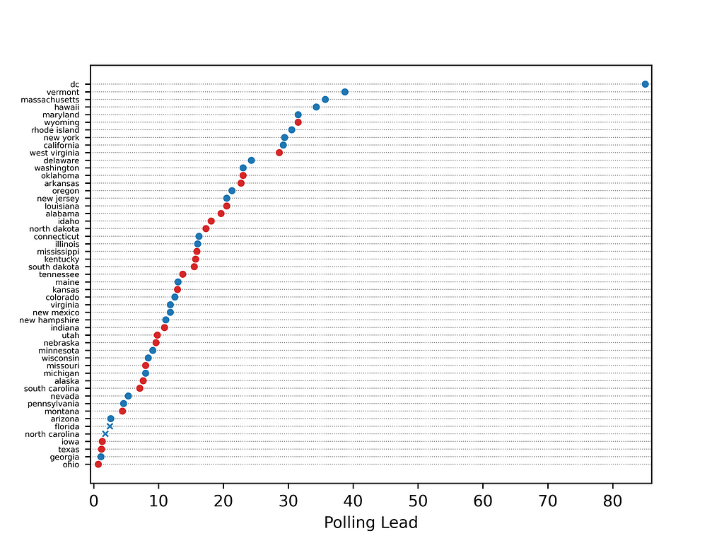
We can see that the leading candidate won in most states, except for North Carolina and Florida.
Let’s fit our Bayesian logistic regression model to the data.
from bbai.glm import BayesianLogisticRegression1

x_2020, y_2020 = # data set for 2020 polls

# We specify w_min so that the prior on w is restricted
# to [0, ∞]; thus, we assume a lead in polls will never
# decrease the probability of the candidate winning the
# state
model = BayesianLogisticRegression1(w_min=0)

model.fit(x_2020, y_2020)
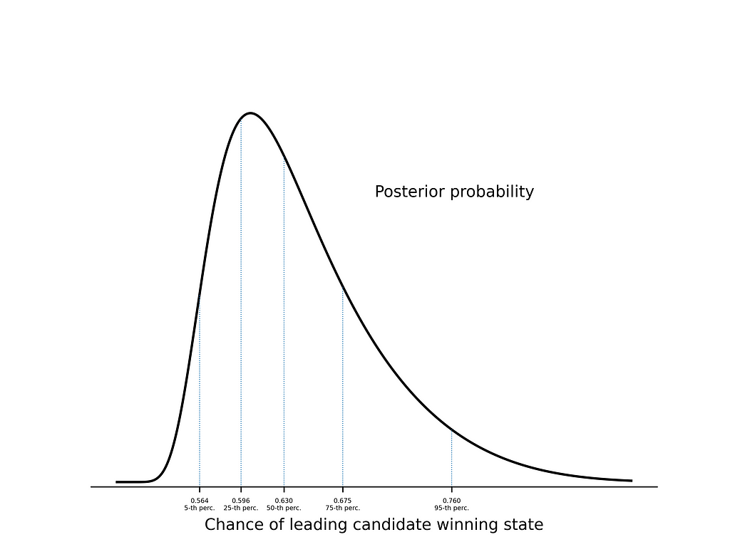
To get a sense for what the model says, we’ll look at how a lead of +1% in state polls translates to the probability of winning the state. Using the posterior distribution, we can look at different percentiles — this gives us a way to quantify our uncertainty in how predictive the polls are:
pred = model.predict(1) # prediction for a 1% polling lead

for pct in [.5, .25, .5, .75, .95]:
    # Use the percentage point function (ppf) to
    # find the value of p where
    #   integrate_0^p π(p | xp=1, x, y) dp = pct
    # Here p denotes the probability of the candidate
    # winning the state when they are leading by +1%.
    print(pct, ':', pred.ppf(pct))
Running the code, we get the result
- 5% of the time, we expect polls to be less predictive than a +1% lead translating to a probability of 0.564 of winning the state
- 25% of the time, we expect polls to be less predictive than a +1% lead translating to a probability of 0.596 of winning the state
- 50% of the time, we expect polls to be less predictive than a +1% lead translating to a probability of 0.630 of winning the state
- 75% of the time, we expect polls to be less predictive than a +1% lead translating to a probability of 0.675 of winning the state
- 95% of the time, we expect polls to be less predictive than a +1% lead translating to a probability of 0.760 of winning the state
Full source code for model: https://github.com/rnburn/bbai/blob/master/example/23-election-polls.ipynb
Now, let’s look at the 2016 election.
2016 Election
Below are FiveThirtyEight’s polling averages for 2016:
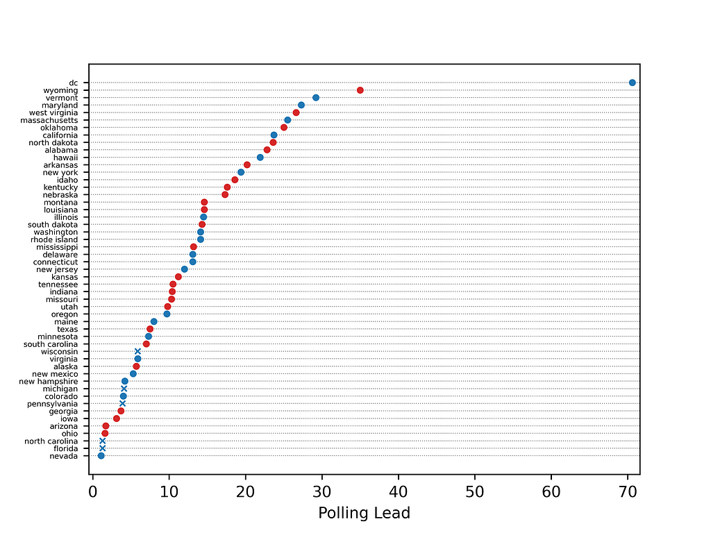
We can see that polls were less accurate in this election. In five cases, the leading candidate lost.
Similarly to 2020, let’s fit our model and look at what it tells us about a +1% polling lead.
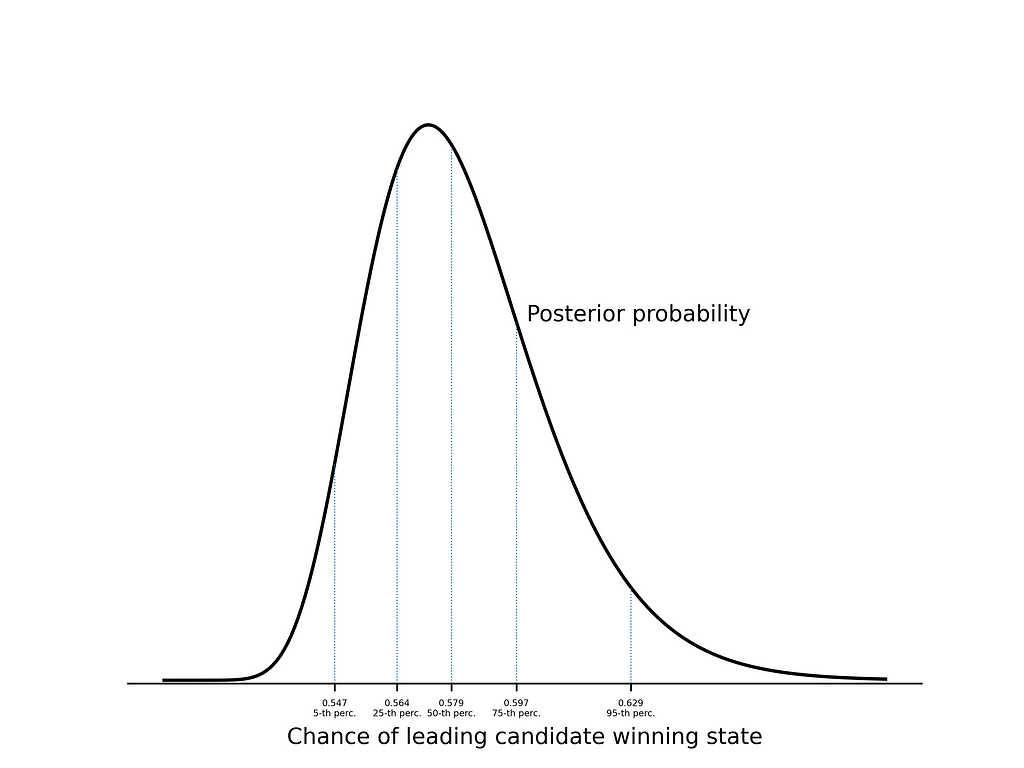
As expected, the model tells us that a 1% polling lead will be less predictive than in 2020.
Full source code for model: https://github.com/rnburn/bbai/blob/master/example/23-election-polls.ipynb
Now, let’s combine the data sets and look at what the models say for some current poll snapshots.
Prediction Snapshots
In the table below, I look at three logistic regression models built using the 2016 data set, the 2020 data set, and the combined 2016 and 2020 data sets. For each model, I give predictions percentiles for a few states using FiveThirtyEight polling averages on 10/20/24 ([6]).

Conclusion
There’s an unfortunate misconception that Bayesian statistics is primarily a subjective discipline and that it’s necessary for a Bayesianist to make arbitrary or controversial choices in prior before they can proceed with an analysis.
In this post, we saw how frequentist matching coverage gives us a natural way to quantify what it means for a prior to represent “knowing nothing”, and we saw how reference analysis gives us a mechanism to build a prior that is, in a certain sense, optimal under frequentist matching coverage given the assumed model.
And once we have the prior, Bayesian statistics provides us with the tools to easily reason about and bound the range of likely prediction possibilities under the model, giving us an easy way to express our uncertainty.
References
[1]: 2020 FiveThirtyEight state-wide polling averages. https://projects.fivethirtyeight.com/polls/president-general/2020/.
Note: FiveThirtyEight allows for reuse of their data with attribution. From https://data.fivethirtyeight.com/:
Unless otherwise noted, our data sets are available under the Creative Commons Attribution 4.0 International license, and the code is available under the MIT license. If you find this information useful, please let us know.
[2]: 2016 FiveThirtyEight state-wide polling averages. https://projects.fivethirtyeight.com/2016-election-forecast/
[3]: Berger, J., J. Bernardo, and D. Sun (2024). Objective Bayesian Inference. World Scientific.
[4]: Berger, J., J. Bernardo, and D. Sun (2022). Objective bayesian inference and its relationship to frequentism.
[5]: Welch, B. L. and H. W. Peers (1963). On formulae for confidence points based on integrals of weighted likelihoods. Journal of the Royal Statistical Society Series B-methodological 25, 318–329.
[6]: 2025 FiveThirtyEight state-wide polling averages. https://projects.fivethirtyeight.com/2024-election-forecast/
Using Objective Bayesian Inference to Interpret Election Polls was originally published in Towards Data Science on Medium, where people are continuing the conversation by highlighting and responding to this story.
from Datascience in Towards Data Science on Medium https://ift.tt/UY46gKt
via IFTTT


