Multimodal Embeddings: An Introduction
Mapping text and images into a common space
This is the 2nd article in a larger series on multimodal AI. In the previous post, we saw how to augment large language models (LLMs) to understand new data modalities (e.g., images, audio, video). One such approach relied on encoders that generate vector representations (i.e. embeddings) of non-text data. In this article, I will discuss multimodal embeddings and share what they can do via two practical use cases.
AI research is traditionally split into distinct fields: NLP, computer vision (CV), robotics, human-computer interface (HCI), etc. However, countless practical tasks require the integration of these different research areas e.g. autonomous vehicles (CV + robotics), AI agents (NLP + CV + HCI), personalized learning (NLP + HCI), etc.
Although these fields aim to solve different problems and work with different data types, they all share a fundamental process. Namely, generating useful numerical representations of real-world phenomena.
Historically, this was done by hand. This means that researchers and practitioners would use their (or other people’s) expertise to explicitly transform data into a more helpful form. Today, however, these can be derived another way.
Embeddings
Embeddings are (useful) numerical representations of data learned implicitly through model training. For example, through learning how to predict text, BERT learned representations of text, which are helpful for many NLP tasks [1]. Another example is the Vision Transformer (ViT), trained for image classification on Image Net, which can be repurposed for other applications [2].
A key point here is that these learned embedding spaces will have some underlying structure so that similar concepts are located close together. As shown in the toy examples below.
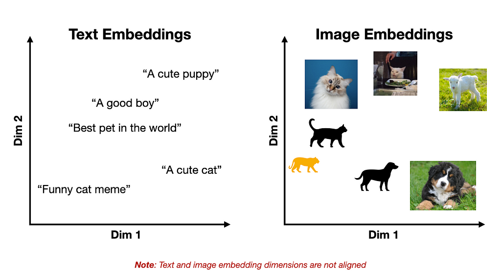
One key limitation of the previously mentioned models is they are restricted to a single data modality, e.g., text or images. Preventing cross-modal applications like image captioning, content moderation, image search, and more. But what if we could merge these two representations?
Multimodal Embeddings
Although text and images may look very different to us, in a neural network, these are represented via the same mathematical object, i.e., a vector. Therefore, in principle, text, images, or any other data modality can processed by a single model.
This fact underlies multimodal embeddings, which represent multiple data modalities in the same vector space such that similar concepts are co-located (independent of their original representations).
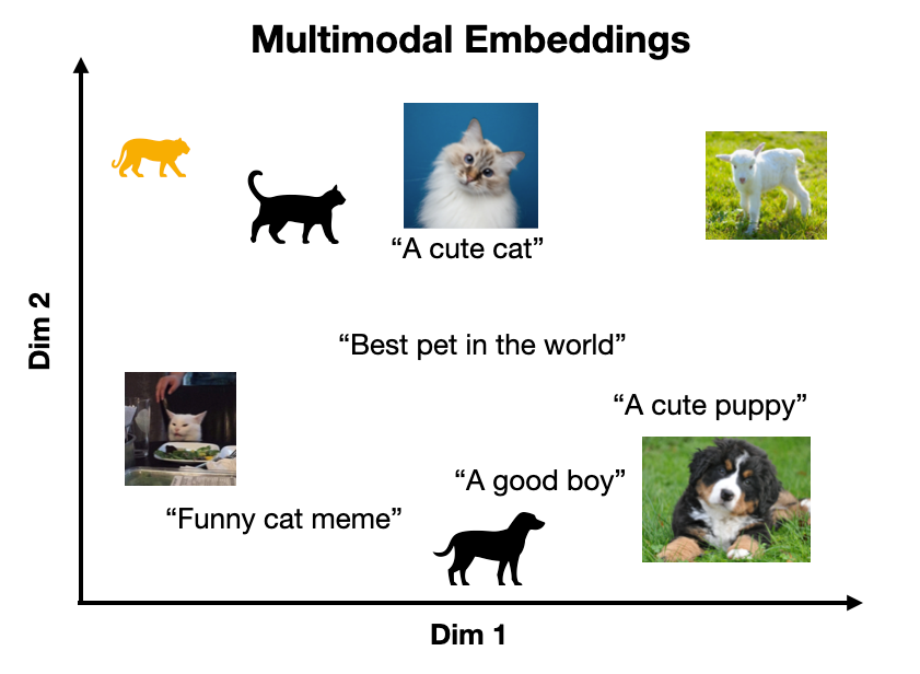
For example, CLIP encodes text and images into a shared embedding space [3]. A key insight from CLIP is that by aligning text and image representations, the model is capable of 0-shot image classification on an arbitrary set of target classes since any input text can be treated as a class label (we will see a concrete example of this later).
However, this idea is not limited to text and images. Virtually any data modalities can be aligned in this way e.g., text-audio, audio-image, text-EEG, image-tabular, and text-video. Unlocking use cases such as video captioning, advanced OCR, audio transcription, video search, and EEG-to-text [4].
Contrastive Learning
The standard approach to aligning disparate embedding spaces is contrastive learning (CL). A key intuition of CL is to represent different views of the same information similarly [5].
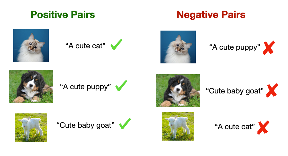
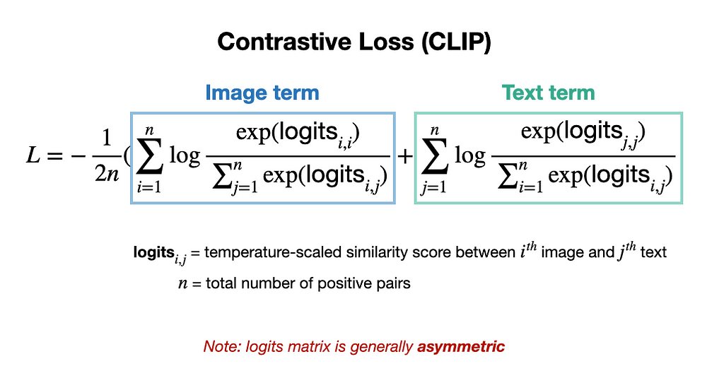
This consists of learning representations that maximize the similarity between positive pairs and minimize the similarity of negative pairs. In the case of an image-text model, a positive pair might be an image with an appropriate caption, while a negative pair would be an image with an irrelevant caption (as shown below).
Two key aspects of CL contribute to its effectiveness
- Since positive and negative pairs can be curated from the data’s inherent structure (e.g., metadata from web images), CL training data do not require manual labeling, which unlocks larger-scale training and more powerful representations [3].
- It simultaneously maximizes positive and minimizes negative pair similarity via a special loss function, as demonstrated by CLIP [3].
Example Code: Using CLIP for 0-shot classification and image search
With a high-level understanding of how multimodal embeddings work, let’s see two concrete examples of what they can do. Here, I will use the open-source CLIP model to perform two tasks: 0-shot image classification and image search.
The code for these examples is freely available on the GitHub repository.
Use case 1: 0-shot Image Classification
The basic idea behind using CLIP for 0-shot image classification is to pass an image into the model along with a set of possible class labels. Then, a classification can be made by evaluating which text input is most similar to the input image.
We’ll start by importing the Hugging Face Transformers library so that the CLIP model can be downloaded locally. Additionally, the PIL library is used to load images in Python.
from transformers import CLIPProcessor, CLIPModel
from PIL import Image
Next, we can import a version of the clip model and its associated data processor. Note: the processor handles tokenizing input text and image preparation.
# import model
model = CLIPModel.from_pretrained("openai/clip-vit-base-patch16")

# import processor (handles text tokenization and image preprocessing)
processor = CLIPProcessor.from_pretrained("openai/clip-vit-base-patch16")
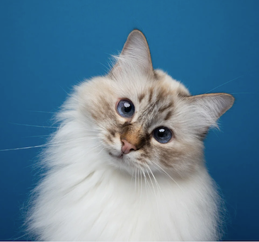
We load in the below image of a cat and create a list of two possible class labels: “a photo of a cat” or “a photo of a dog”.
# load image
image = Image.open("images/cat_cute.png")

# define text classes
text_classes = ["a photo of a cat", "a photo of a dog"]
Next, we’ll preprocess the image/text inputs and pass them into the model.
# pass image and text classes to processor
inputs = processor(text=text_classes, images=image, return_tensors="pt",
                                                    padding=True)

# pass inputs to CLIP
outputs = model(**inputs) # note: "**" unpacks dictionary items
To make a class prediction, we must extract the image logits and evaluate which class corresponds to the maximum.
# image-text similarity score
logits_per_image = outputs.logits_per_image
# convert scores to probs via softmax
probs = logits_per_image.softmax(dim=1)

# print prediction
predicted_class = text_classes[probs.argmax()]
print(predicted_class, "| Probability = ",
                       round(float(probs[0][probs.argmax()]),4))
>> a photo of a cat | Probability = 0.9979
The model nailed it with a 99.79% probability that it’s a cat photo. However, this was a super easy one. Let’s see what happens when we change the class labels to: “ugly cat” and “cute cat” for the same image.
>> cute cat | Probability = 0.9703
The model easily identified that the image was indeed a cute cat. Let’s do something more challenging like the labels: “cat meme” or “not cat meme”.
>> not cat meme | Probability = 0.5464
While the model is less confident about this prediction with a 54.64% probability, it correctly implies that the image is not a meme.
Use case 2: Image Search
Another application of CLIP is essentially the inverse of Use Case 1. Rather than identifying which text label matches an input image, we can evaluate which image (in a set) best matches a text input (i.e. query)—in other words, performing a search over images.
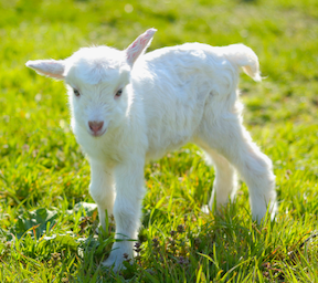
We start by storing a set of images in a list. Here, I have three images of a cat, dog, and goat, respectively.
# create list of images to search over
image_name_list = ["images/cat_cute.png", "images/dog.png", "images/goat.png"]

image_list = []
for image_name in image_name_list:
    image_list.append(Image.open(image_name))
Next, we can define a query like “a cute dog” and pass it and the images into CLIP.
# define a query
query = "a cute dog"

# pass images and query to CLIP
inputs = processor(text=query, images=image_list, return_tensors="pt",
                                                  padding=True)
We can then match the best image to the input text by extracting the text logits and evaluating the image corresponding to the maximum.
# compute logits and probabilities
outputs = model(**inputs)
logits_per_text = outputs.logits_per_text
probs = logits_per_text.softmax(dim=1)

# print best match
best_match = image_list[probs.argmax()]
prob_match = round(float(probs[0][probs.argmax()]),4)

print("Match probability: ",prob_match)
display(best_match)
>> Match probability: 0.9817
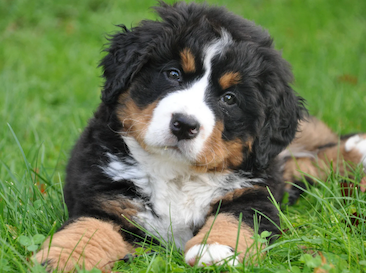
We see that (again) the model nailed this simple example. But let’s try some trickier examples.
query = "something cute but metal 🤘"
>> Match probability: 0.7715
query = "a good boy"
>> Match probability: 0.8248

query = "the best pet in the world"
>> Match probability: 0.5664

Although this last prediction is quite controversial, all the other matches were spot on! This is likely since images like these are ubiquitous on the internet and thus were seen many times in CLIP’s pre-training.
YouTube-Blog/multimodal-ai/2-mm-embeddings at main · ShawhinT/YouTube-Blog
What’s Next?
Multimodal embeddings unlock countless AI use cases that involve multiple data modalities. Here, we saw two such use cases, i.e., 0-shot image classification and image search using CLIP.
Another practical application of models like CLIP is multimodal RAG, which consists of the automated retrieval of multimodal context to an LLM. In the next article of this series, we will see how this works under the hood and review a concrete example.
More on Multimodal models 👇
My website: https://www.shawhintalebi.com/
- [1] BERT
- [2] ViT
- [3] CLIP
- [4] Thought2Text: Text Generation from EEG Signal using Large Language Models (LLMs)
- [5] A Simple Framework for Contrastive Learning of Visual Representations
Multimodal Embeddings: An Introduction was originally published in Towards Data Science on Medium, where people are continuing the conversation by highlighting and responding to this story.
from Datascience in Towards Data Science on Medium https://ift.tt/18QXmPH
via IFTTT


